api

High-level API for bpf4

The API allows a high-level and flexible interface to the core of bpf4, which is implemented in cython for efficiency.

API vs core

These three curves, a, b and c define the same linear break-point-function The first two definitions, a and b, use the high-level API, which allows for points to be defined as a flat sequence, as tuples of (x, y). The core classes need to be instantiated with two arrays of x and y values, as in c

from bpf4 import *
a = linear(0, 0, 1, 2.5, 3, 10)
b = linear((0, 0), (1, 2.5), (3, 10))
c = core.Linear([0, 1, 3], [0, 2.5, 10])

---

Function	Description
blendshape	Create a bpf blending two interpolation forms
const	A bpf which always returns a constant value
expon	Construct an Expon bpf (a bpf with exponential interpolation)
halfcos	Construct a half-cosine bpf (a bpf with half-cosine interpolation)
halfcosexp	Construct a half-cosine bpf (a bpf with half-cosine interpolation)
halfcosm	Halfcos interpolation with symmetric exponent
linear	Construct a Linear bpf.
multi	A bpf with a per-pair interpolation
nearest	A bpf with floor interpolation
nointerpol	A bpf with floor interpolation
pchip	Monotonic Cubic Hermite Intepolation
slope	Generate a straight line with the given slope and offset
smooth	A bpf with smoothstep interpolation.
smoother	A bpf with smootherstep interpolation
spline	Construct a cubic-spline bpf
stack	A bpf representing a stack of bpf
uspline	Construct a univariate cubic-spline bpf

---

blendshape

def blendshape(shape0: str, shape1: str, mix: float | core.BpfInterface, points
               ) -> core.BpfInterface

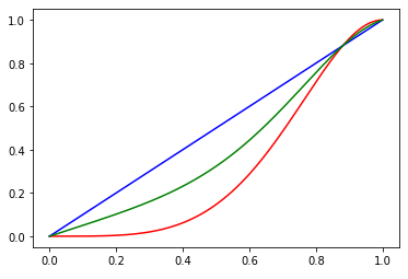
Create a bpf blending two interpolation forms

Example

from bpf4 import *
a = blendshape('halfcos(2.0)', 'linear', mix=0.5, points=(0, 0, 1, 1))
halfcos(0, 0, 1, 1, exp=2).plot(color='red')
linear(0, 0, 1, 1).plot(color='blue')
a.plot(color='green')

Args

• shape0 (str): a description of the first interpolation
• shape1 (str): a description of the second interpolation
• mix (float | core.BpfInterface): blend factor. A value between 0 (use only shape0) and 1 (use only shape1). A value of 0.5 will result in an average between the first and second interpolation kind. Can be a bpf itself, returning the mix value at any x value
• points: either a tuple (x0, y0, x1, y1, ...) or a tuple (xs, ys) where xs and ys are lists/arrays containing the x and y coordinates of the points

Returns

    (core.BpfInterface) A bpf blending two different interpolation kinds

---

const

def const(value) -> core.Const

A bpf which always returns a constant value

Example

>>> c5 = const(5)
>>> c5(10) 
5

Args

• value: the constant value

---

expon

def expon(args, kws) -> core.Expon

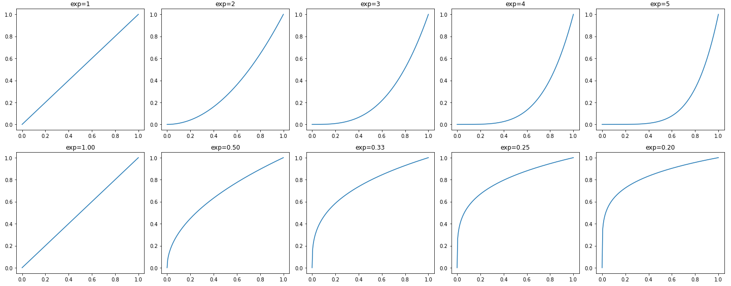
Construct an Expon bpf (a bpf with exponential interpolation)

A bpf can be constructed in multiple ways:

expon(x0, y0, x1, y1, ..., exp=exponent)
expon(exponent, x0, y0, x1, y1, ...)
expon((x0, y0), (x1, y1), ..., exp=exponent)
expon({x0:y0, x1:y1, ...}, exp=exponent)

Example

from bpf4 import *
import matplotlib.pyplot as plt
numplots = 5
fig, axs = plt.subplots(2, numplots, tight_layout=True, figsize=(20, 8))
for i in range(numplots):
    exp = i+1
    expon(0, 0, 1, 1, exp=exp).plot(show=False, axes=axs[0, i])
    expon(0, 0, 1, 1, exp=1/exp).plot(show=False, axes=axs[1, i])
    axs[0, i].set_title(f'{exp=}')
    axs[1, i].set_title(f'exp={1/exp:.2f}')

plot.show()

Args

• args: either a flat list of coordinates in the form x0, y0, x1, y1, ..., a list of tuples (x0, y0), (x1, y1), ..., a dict {x0:y0, x1:y1, ...} or two arrays xs and ys
• kws:

---

halfcos

def halfcos(args, exp: int = 1, numiter: int = 1, kws) -> core.Halfcos

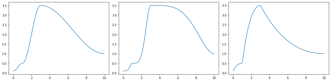
Construct a half-cosine bpf (a bpf with half-cosine interpolation)

A bpf can be constructed in multiple ways:

halfcos(x0, y0, x1, y1, ...)
halfcos((x0, y0), (x1, y1), ...)
halfcos({x0:y0, x1:y1, ...})

a = halfcos([0, 1, 3, 10], [0.1, 0.5, 3.5,  1])
b = halfcos(*a.points(), exp=2)
c = halfcos(*a.points(), exp=0.5)
fig, axes = plt.subplots(1, 3, figsize=(16, 4), tight_layout=True)
a.plot(axes=axes[0], show=False)
b.plot(axes=axes[1], show=False)
c.plot(axes=axes[2])

Args

• args: either a flat list of coordinates in the form x0, y0, x1, y1, ..., a list of tuples (x0, y0), (x1, y1), ..., a dict {x0:y0, x1:y1, ...} or two arrays xs and ys
• exp (int): the exponent to use (default: 1)
• numiter (int): Number of iterations. A higher number accentuates the effect (default: 1)
• kws:

---

halfcos

def halfcos(args, exp: int = 1, numiter: int = 1, kws) -> core.Halfcos

Construct a half-cosine bpf (a bpf with half-cosine interpolation)

A bpf can be constructed in multiple ways:

halfcos(x0, y0, x1, y1, ...)
halfcos((x0, y0), (x1, y1), ...)
halfcos({x0:y0, x1:y1, ...})

a = halfcos([0, 1, 3, 10], [0.1, 0.5, 3.5,  1])
b = halfcos(*a.points(), exp=2)
c = halfcos(*a.points(), exp=0.5)
fig, axes = plt.subplots(1, 3, figsize=(16, 4), tight_layout=True)
a.plot(axes=axes[0], show=False)
b.plot(axes=axes[1], show=False)
c.plot(axes=axes[2])

Args

• args: either a flat list of coordinates in the form x0, y0, x1, y1, ..., a list of tuples (x0, y0), (x1, y1), ..., a dict {x0:y0, x1:y1, ...} or two arrays xs and ys
• exp (int): the exponent to use (default: 1)
• numiter (int): Number of iterations. A higher number accentuates the effect (default: 1)
• kws:

---

halfcosm

def halfcosm(args, kws) -> core.Halfcosm

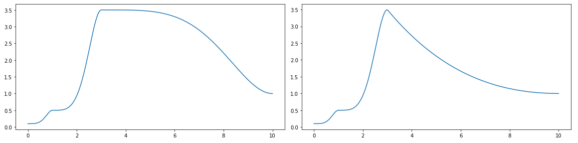
Halfcos interpolation with symmetric exponent

When used with an exponent, the exponent is inverted for downwards segments (y1 > y0)

A bpf can be constructed in multiple ways:

halfcosm(x0, y0, x1, y1, ..., exp=2.0)
halfcosm(2.0, x0, y0, x1, y1, ...)    # The exponent can be placed first
halfcosm((x0, y0), (x1, y1), ...)
halfcosm({x0:y0, x1:y1, ...})

from bpf4 import *
a = halfcosm(0, 0.1,
             1, 0.5,
             3, 3.5,
             10, 1, exp=2)
b = halfcosm(*a.points(), exp=2)
fig, axes = plt.subplots(1, 2, figsize=(16, 4))
a.plot(axes=axes[0], show=False)
b.plot(axes=axes[1])

Args

• args: either a flat list of coordinates in the form x0, y0, x1, y1, ..., a list of tuples (x0, y0), (x1, y1), ..., a dict {x0:y0, x1:y1, ...} or two arrays xs and ys
• kws:

Returns

    (core.Halfcosm) A bpf with symmetric cosine interpolation

---

linear

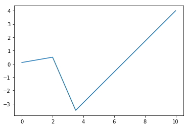
def linear(args) -> core.Linear

Construct a Linear bpf.

A bpf can be constructed in multiple ways, all of which result in the same Linear instance:

linear(x0, y0, x1, y1, ...)
linear((x0, y0), (x1, y1), ...)
linear({x0:y0, x1:y1, ...})

Example

from bpf4 import *
a = linear([0, 2, 3.5, 10], [0.1, 0.5, -3.5,  4])
a.plot()

Args

• args: either a flat list of coordinates in the form x0, y0, x1, y1, ..., a list of tuples (x0, y0), (x1, y1), ..., a dict {x0:y0, x1:y1, ...} or two arrays xs and ys

---

multi

def multi(args) -> None

A bpf with a per-pair interpolation

Example

# (0,0) --linear-- (1,10) --expon(3)-- (2,3) --expon(3)-- (10, -1) --halfcos-- (20,0)

multi(0, 0,   'linear' 
      1, 10,  'expon(3)', 
      2, 3,   # assumes previous interpolation 
      10, -1, 'halfcos'      
      20, 0)

# also the following syntax is possible
multi((0, 0, 'linear')
      (1, 10, 'expon(3)'), 
      (2, 3), 
      (10, -1, 'halfcos'), 
      (20, 0))

Args

• args:

---

nearest

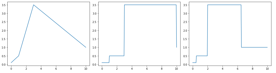
def nearest(args) -> core.Nearest

A bpf with floor interpolation

A bpf can be constructed in multiple ways:

nearest(x0, y0, x1, y1, ...)
nearest((x0, y0), (x1, y1), ...)
nearest({x0:y0, x1:y1, ...})

a = linear([0, 1, 3, 10], [0.1, 0.5, 3.5,  1])
b = nointerpol(*a.points())
c = nearest(*a.points())
fig, axes = plt.subplots(1, 3, figsize=(15, 4), tight_layout=True)
a.plot(axes=axes[0], show=False)
b.plot(axes=axes[1], show=False)
c.plot(axes=axes[2])

Args

• args: either a flat list of coordinates in the form x0, y0, x1, y1, ..., a list of tuples (x0, y0), (x1, y1), ..., a dict {x0:y0, x1:y1, ...} or two arrays xs and ys

---

nointerpol

def nointerpol(args) -> core.NoInterpol

A bpf with floor interpolation

A bpf can be constructed in multiple ways:

nointerpol(x0, y0, x1, y1, ...)
nointerpol((x0, y0), (x1, y1), ...)
nointerpol({x0:y0, x1:y1, ...})

a = linear([0, 1, 3, 10], [0.1, 0.5, 3.5,  1])
b = nointerpol(*a.points())
c = nearest(*a.points())
fig, axes = plt.subplots(1, 3, figsize=(15, 4), tight_layout=True)
a.plot(axes=axes[0], show=False)
b.plot(axes=axes[1], show=False)
c.plot(axes=axes[2])

Args

• args: either a flat list of coordinates in the form x0, y0, x1, y1, ..., a list of tuples (x0, y0), (x1, y1), ..., a dict {x0:y0, x1:y1, ...} or two arrays xs and ys

---

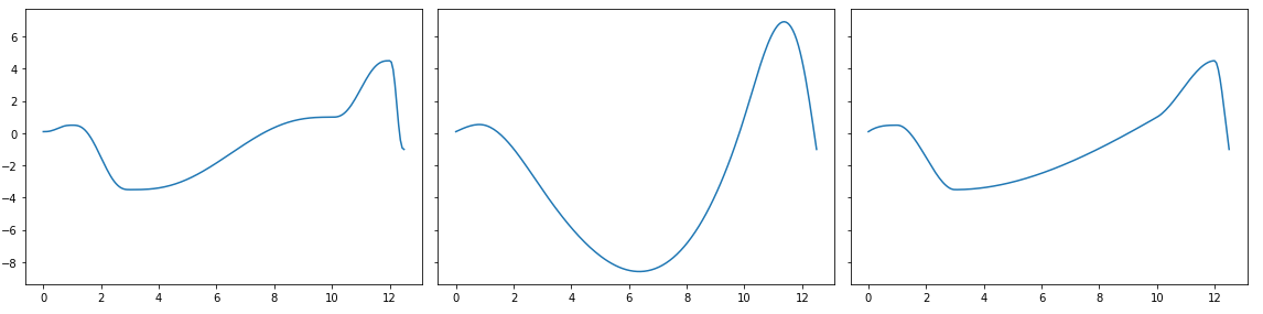
pchip

def pchip(args) -> None

Monotonic Cubic Hermite Intepolation

A bpf can be constructed in multiple ways:

pchip(x0, y0, x1, y1, ...)
pchip((x0, y0), (x1, y1), ...)
pchip({x0:y0, x1:y1, ...})


>>> a = core.Smoother([0, 1, 3, 10, 12, 12.5], [0.1, 0.5, -3.5,  1, 4.5, -1])
>>> b = core.Spline(*a.points())
>>> c = pchip(*a.points())

>>> fig, axes = plt.subplots(1, 3, figsize=(16, 4), sharey=True, tight_layout=True)
>>> a.plot(axes=axes[0], show=False)
>>> b.plot(axes=axes[1], show=False)
>>> c.plot()

Args

• args: either a flat list of coordinates in the form x0, y0, x1, y1, ..., a list of tuples (x0, y0), (x1, y1), ..., a dict {x0:y0, x1:y1, ...} or two arrays xs and ys

---

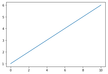
slope

def slope(slope: float, offset: float = 0.0, bounds: tuple[float, float] = None
          ) -> core.Slope

Generate a straight line with the given slope and offset

This is the same as linear(0, offset, 1, slope)

Example

>>> a = slope(0.5, 1)
>>> a
Slope[-inf:inf]
>>> a[0:10].plot()

Args

• slope (float):
• offset (float): (default: 0.0)
• bounds (tuple[float, float]): (default: None)

---

smooth

def smooth(args, numiter: int = 1) -> core.Smooth

A bpf with smoothstep interpolation.

from bpf4.api import *
a = smooth((0, 0.1), (1, 0.5), (3, -3.5), (10, 1))
a.plot()

See Also

• smoother

Args

• args: either a flat list of coordinates in the form x0, y0, x1, y1, ..., a list of tuples (x0, y0), (x1, y1), ..., a dict {x0:y0, x1:y1, ...} or two arrays xs and ys
• numiter (int): determines the number of smoothstep steps applied (see https://en.wikipedia.org/wiki/Smoothstep) (default: 1)

Returns

    (core.Smooth) A bpf with smoothstep interpolation

---

smoother

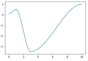
def smoother(args) -> core.Smoother

A bpf with smootherstep interpolation

This bpf uses Perlin's variation on smoothstep, see https://en.wikipedia.org/wiki/Smoothstep)

from bpf4 import *
a = smooth(0, 0.1, 
           1, 0.5, 
           3, -3.5, 
           10, 1)
b = smoother(*a.points())
fig, axes = plt.subplots(1, 2, figsize=(12, 4))
a.plot(axes=axes[0], show=False)
b.plot(axes=axes[1])

Args

• args: either a flat list of coordinates in the form x0, y0, x1, y1, ..., a list of tuples (x0, y0), (x1, y1), ..., a dict {x0:y0, x1:y1, ...} or two arrays xs and ys

Returns

    (core.Smoother) A bpf with smootherstep interpolation

---

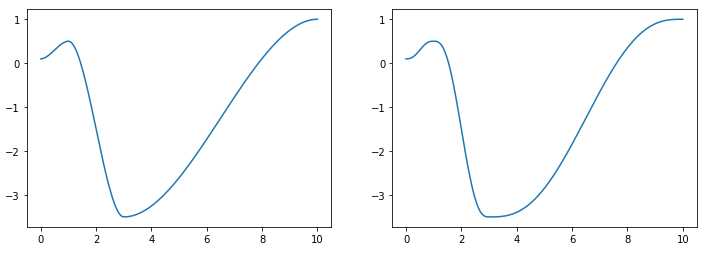
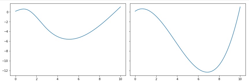
spline

def spline(args) -> core.Spline

Construct a cubic-spline bpf

A bpf can be constructed in multiple ways:

spline(x0, y0, x1, y1, ...)
spline((x0, y0), (x1, y1), ...)
spline({x0:y0, x1:y1, ...})

from bpf4 import *
a = smooth(0, 0.1, 1, 0.5, 3, -3.5, 10, 1)
b = spline(*a.points())
fig, axes = plt.subplots(1, 2, figsize=(12, 4))
a.plot(axes=axes[0], show=False)
b.plot(axes=axes[1])

Args

• args: either a flat list of coordinates in the form x0, y0, x1, y1, ..., a list of tuples (x0, y0), (x1, y1), ..., a dict {x0:y0, x1:y1, ...} or two arrays xs and ys

Returns

    (core.Spline) A Spline bpf

---

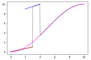
stack

def stack(bpfs) -> core.Stack

A bpf representing a stack of bpf

Within a Stack, a bpf does not have outbound values. When evaluated outside its bounds the bpf below is used, iteratively until the lowest bpf is reached. Only the lowest bpf is evaluated outside its bounds

Example

# Interval    bpf
# [0, 3]      a
# (3, 4]      b
# (4, 10]     c

from bpf4 import *
import matplotlib.pyplot as plt
a = linear(0, 0, 3, 1)
b = linear(2, 9, 4, 10)
c = halfcos(0, 0, 10, 10)
s = core.Stack((a, b, c))

ax = plt.subplot(111)
a.plot(color="#f00", alpha=0.4, axes=ax, linewidth=4, show=False)
b.plot(color="#00f", alpha=0.4, axes=ax, linewidth=4, show=False)
c.plot(color="#f0f", alpha=0.4, axes=ax, linewidth=4, show=False)
s.plot(axes=ax, linewidth=2, color="#000", linestyle='dotted')

Args

• bpfs: a sequence of bpfs

Returns

    (core.Stack) A stacked bpf

---

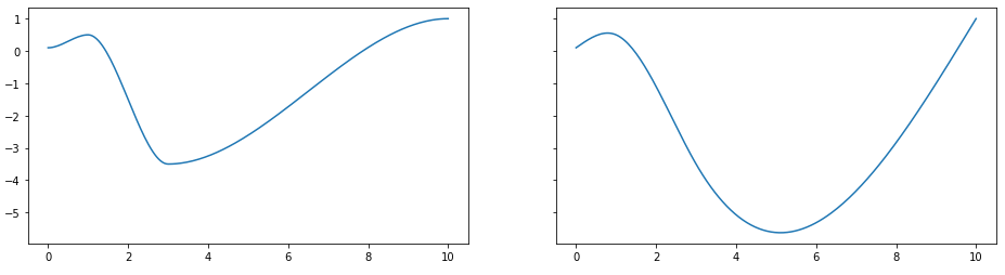
uspline

def uspline(args) -> core.USpline

Construct a univariate cubic-spline bpf

A bpf can be constructed in multiple ways:

uspline(x0, y0, x1, y1, ...)
uspline((x0, y0), (x1, y1), ...)
uspline({x0:y0, x1:y1, ...})

from bpf4 import *
a = spline(0, 0.1, 1, 0.5, 3, -3.5, 10, 1)
b = uspline(*a.points())

fig, axes = plt.subplots(1, 2, figsize=(12, 4), sharey=True, tight_layout=True)
a.plot(axes=axes[0], show=False)
b.plot(axes=axes[1])

See Also

• spline
• pchip

Args

• args: either a flat list of coordinates in the form x0, y0, x1, y1, ..., a list of tuples (x0, y0), (x1, y1), ..., a dict {x0:y0, x1:y1, ...} or two arrays xs and ys

Returns

    (core.USpline) A USpline bpf