core

---

Class	Description
BpfBase	BpfBase(xs, ys)
BpfInterface	Base class for all Break-Point Functions
BpfInversionError
BpfPointsError
Const	Const(double value, tuple bounds: tuple[float, float] = None)
Expon	Expon(xs, ys, double exp, int numiter=1)
Exponm	Exponm(xs, ys, double exp, int numiter=1)
Halfcos	Halfcos(xs, ys, double exp=1.0, int numiter=1)
HalfcosExp	Halfcos(xs, ys, double exp=1.0, int numiter=1)
Halfcosm	Halfcosm(xs, ys, double exp=1.0, int numiter=1)
Linear	Linear(xs, ys)
Max	Max(*bpfs)
Min	Min(*bpfs)
Multi	Multi(xs, ys, interpolations)
NanMask	NanMask(BpfInterface a, double masked=0.)
Nearest	Nearest(xs, ys)
NoInterpol	NoInterpol(xs, ys)
Sampled	Sampled(samples, double dx, double x0=0, unicode interpolation=u'linear')
Slope	Slope(double slope, double offset=0, tuple bounds=None)
Smooth	Smooth(xs, ys, int numiter=1)
Smoother	Smoother(xs, ys)
Spline	Spline(xs, ys)
Stack	Stack(bpfs)
USpline	USpline(xs, ys)

Function	Description
blend	Blend these BPFs
bpf_zero_crossings	Return the zeros if b in the interval defined
brentq	Calculate the zero of bpf + x0 in the interval (xa, xb) using brentq algorithm
setA4	Set the reference freq used

---

BpfInterface

def () -> None

Base class for all Break-Point Functions

Note

BpfInterace is an abstract class. It is not possible to create an instance of it.

---

Summary

Property	Description
x0	BpfInterface.x0: float
The lower bound of the x coordinate
x1	BpfInterface.x1: float
The upper bound of the x coordinate

Method	Description
abs	Returns a bpf representing the absolute value of this bpf
acos	Returns a bpf representing the arc cosine of this bpf
amp2db	Returns a bpf converting linear amplitudes to decibels
apply	Create a bpf where func is applied to the result of this pdf
asin	Returns a bpf representing the arc sine of this bpf
bounds	Returns a tuple (xstart, xend) representing the bounds of this bpf
ceil	Returns a bpf representing the ceil of this bpf
clip	Return a bpf clipping the result between y0 and y1
concat	Concatenate this bpf to other
copy	Create a copy of this bpf
cos	Returns a bpf representing the cosine of this bpf
crop	Crop this bpf at the given x values (x0, x1)
db2amp	Returns a bpf converting decibels to linear amplitudes
derivative	Create a curve which represents the derivative of this curve
dxton	Split the bounds of this bpf according to a given sampling period dx
expon	Returns a bpf representing the exp operation with this bpf
f2m	Returns a bpf converting frequencies to midinotes
fit_between	Returns a view of this bpf fitted within the interval x0:x1
floor	Returns a bpf representing the floor of this bpf
fromseq	BpfInterface.fromseq(cls, points, *kws)
integrate	Return the result of the integration of this bpf.
integrate_between	Integrate this bpf between x0 and x1
integrated	Return a bpf representing the integration of this bpf at a given point
inverted	Return a view on this bpf with the coords inverted
keep_slope	A view of this bpf where the slope is continued outside its bounds
log	Returns a bpf representing the log of this bpf
log10	Returns a bpf representing the log10 of this bpf
m2f	Returns a bpf converting from midinotes to frequency
map	The same as map(self, xs) but faster
mapn_between	Calculate an array of n values representing this bpf between x0 and x1
max	Returns a bpf representing max(self, b)
mean	Calculate the mean value of this bpf.
min	Returns a bpf representing min(self, b)
nanmask	A nan mask from this bpf
ntodx	Calculate the sampling period dx
outbound	Return a new Bpf with the given values outside the bounds
periodic	Create a new bpf which replicates this in a periodic way
plot	Plot the bpf using matplotlib.pyplot. Any key is passed to plot.plot_coords
preapply	Create a bpf where func is applied to the argument before it is passed
rand	A bpf representing rand(self(x))
render	Create a new bpf representing this bpf rendered at the given points
round	A bpf representing round(self(x))
sample_between	Sample this bpf at an interval of dx between x0 and x1
sampled	Sample this bpf at a regular interval, returns a Sampled bpf
sampled_between	Sample a portion of this bpf, returns a Sampled bpf
shifted	Returns a view of this bpf shifted by dx over the x-axes
sin	Returns a bpf representing the sine of this bpf
sinh	Returns a bpf representing the sinh of this bpf
sqrt	Returns a bpf representing the sqrt of this bpf
stretched	Returns a view of this bpf stretched over the x axis.
tan	Returns a bpf representing the tan of this bpf
tanh	Returns a bpf representing the tanh of this bpf
zeros	Find the zeros of this bpf

---

Attributes

• x0: BpfInterface.x0: float The lower bound of the x coordinate
• x1: BpfInterface.x1: float The upper bound of the x coordinate

---

Methods

abs

BpfInterface.abs(self) -> _BpfUnaryFunc

Returns a bpf representing the absolute value of this bpf

---

acos

BpfInterface.acos(self) -> _BpfUnaryFunc

Returns a bpf representing the arc cosine of this bpf

---

amp2db

BpfInterface.amp2db(self) -> _Bpf_amp2db

Returns a bpf converting linear amplitudes to decibels

Example

>>> linear(0, 0, 1, 1).amp2db().map(10)
array([-280.        ,  -19.08485019,  -13.06425028,   -9.54242509,
       -7.04365036,   -5.1054501 ,   -3.52182518,   -2.18288939,
       -1.02305045,    0.        ])

Returns

    (BpfInterface) A bpf representing \x -> amp2db(self(x))

---

apply

BpfInterface.apply(self, func)

Create a bpf where func is applied to the result of this pdf

NB: a.apply(b) is the same as a | b

Example

>>> from bpf4 import *
>>> from math import *
>>> a = linear(0, 0, 1, 10)
>>> def func(x):
...     return sin(x) + 1
>>> b = a.apply(func)
>>> b(1)
0.4559788891106302
>>> sin(a(1)) + 1
0.4559788891106302

Args

• func (callable): a function to apply to the result of this bpf

Returns

    (BpfInterface) A bpf representing func(self(x))

---

asin

BpfInterface.asin(self) -> _BpfUnaryFunc

Returns a bpf representing the arc sine of this bpf

---

bounds

BpfInterface.bounds(self)

Returns a tuple (xstart, xend) representing the bounds of this bpf

The returned bounds indicate the range within which this bpf is defined, but any bpf can be evaluated outside those bounds. In such a case the out-of-bound result will depend on the concrete subclass being evaluated. For most cases the out-of-bound result is the same as the result at the bounds

Example

>>> from bpf4 import *
>>> a = linear(1, 10, 2, 25)
>>> a.bounds()
(1.0, 2.0)

Returns

    (tuple[float, float]) The bounbs of this bpf

---

ceil

BpfInterface.ceil(self) -> _BpfUnaryFunc

Returns a bpf representing the ceil of this bpf

---

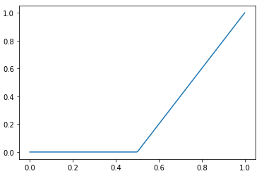
clip

BpfInterface.clip(self, double y0=-inf, double y1=inf) -> _BpfLambdaClip

Return a bpf clipping the result between y0 and y1

>>> a = linear(0, -1, 1, 1).clip(0, 1)
>>> a.map(20)
array([0.        , 0.        , 0.        , 0.        , 0.        ,
       0.        , 0.        , 0.        , 0.        , 0.        ,
       0.05263158, 0.15789474, 0.26315789, 0.36842105, 0.47368421,
       0.57894737, 0.68421053, 0.78947368, 0.89473684, 1.        ])
>>> a.plot()

Args

• y0 (float): the min. y value (default: -inf)
• y1 (float): the max. y value (default: inf)

Returns

    (BpfInterface) A view of this bpf clipped to the given y values

---

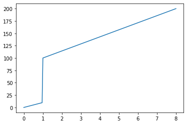
concat

BpfInterface.concat(self, BpfInterface other) -> BpfInterface

Concatenate this bpf to other

other is shifted to start at the end of self

Example

>>> a = linear(0, 0, 1, 10)
>>> b = linear(3, 100, 10, 200)
>>> c = a.concat(b)
>>> c
_BpfConcat2[0.0:8.0]
>>> c(1 - 1e-12), c(1)
(9.99999999999, 100.0)
>>> c.plot()

Args

• other:

---

copy

BpfInterface.copy(self)

Create a copy of this bpf

Returns

    (BpfInterface) A copy of this bpf

---

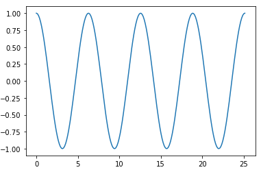
cos

BpfInterface.cos(self) -> _BpfUnaryFunc

Returns a bpf representing the cosine of this bpf

from bpf4 import *
from math import pi
a = slope(1).cos()
a[0:8*pi].plot()

---

crop

BpfInterface.crop(self, double x0, double x1, y0=None, y1=None)

Crop this bpf at the given x values (x0, x1)

Note

This is the same as taking a slice bpf[lowerbound:upperbound] but this method allows to explicitely set the outbound values. These two statements are the same: bpf[x0:x1].outbound(y0, y1) and bpf.slice(x0, x1, y0, y1)

Args

• x0 (float): the lower bound to cut this bpf at
• x1 (float): the upper bound to cut this bpf
• y0 (float): if given, the value returned for x < x0 (default: None)
• y1 (float): if given, the value returned for x > x1 (default: None)

Returns

    (_BpfCrop) this bpf cropped to the interval x0:x1. If y0 and/our y1 are given, then these values are returned for any x outside the given bounds, otherwise the value returned by this bpf at x0 is extended for any x < x0 and the same for the upper bound

---

db2amp

BpfInterface.db2amp(self) -> _Bpf_db2amp

Returns a bpf converting decibels to linear amplitudes

Example

>>> linear(0, 0, 1, -60).db2amp().map(10)
array([1.        , 0.46415888, 0.21544347, 0.1       , 0.04641589,
       0.02154435, 0.01      , 0.00464159, 0.00215443, 0.001     ])

Returns

    (BpfInterface) A bpf representing \x -> db2amp(self(x))

---

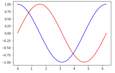
derivative

BpfInterface.derivative(self) -> BpfInterface

Create a curve which represents the derivative of this curve

It implements Newtons difference quotiont, so that:

                bpf(x + h) - bpf(x)
derivative(x) = -------------------
                          h

Example

>>> from bpf4 import *
>>> a = slope(1)[0:6.28].sin()
>>> a.plot(show=False, color="red")
>>> b = a.derivative()
>>> b.plot(color="blue")

Returns

    (BpfInterface) A bpf which returns the derivative of this bpf at any given x coord

---

dxton

BpfInterface.dxton(self, double dx) -> int

Split the bounds of this bpf according to a given sampling period dx

Calculate the number of points in as a result of dividing the bounds of this bpf by the sampling period dx:

n = (x1 + dx - x0) / dx

where x0 and x1 are the x coord start and end points and dx is the sampling period.

>>> from bpf4 import *
>>> a = linear(0, 0, 1,  10, 2, 5)
# Sample a with a period of 0.1
>>> ys = a.map(a.dxton(0.1))
>>> len(ys)
21
>>> ys
array([ 0.,  1.,  2.,  3.,  4.,  5.,  6.,  7.,  8.,  9., 10.,  9.,  8.,
7.,  6.,  5.,  4.,  3.,  2.,  1.,  0.])

See Also

ntodx()

Args

• dx (float): the sampling period

Returns

    (int) The number of points to sample

---

expon

BpfInterface.expon(self) -> _BpfUnaryFunc

Returns a bpf representing the exp operation with this bpf

Example

>>> from bpf4 import *
>>> a = linear(0, 0, 1, 10)
>>> a(0.1)
1.0
>>> exp(1.0)
2.718281828459045
>>> a.expon()(0.1)
2.718281828459045

---

f2m

BpfInterface.f2m(self, double a4=0.)

Returns a bpf converting frequencies to midinotes

Example

>>> from bpf4 import *
>>> freqs = linear(0, 442, 1, 882)
>>> freqs.f2m().map(10)
array([69.        , 70.82403712, 72.47407941, 73.98044999, 75.3661766 ,
       76.64915905, 77.84358713, 78.96089998, 80.01045408, 81.        ])

Args

• a4 (float): frequency value for A4. If not given, uses the global value (see setA4) (default: 0.0)

Returns

    (BpfInterface) A bpf representing \x -> f2m(self(x))

---

fit_between

BpfInterface.fit_between(self, double x0, double x1) -> BpfInterface

Returns a view of this bpf fitted within the interval x0:x1

This operation only makes sense if the bpf is bounded (none of its bounds is inf)

Example

>>> from bpf4 import *
>>> a = linear(1, 1, 2, 5)
>>> a.bounds()
(1, 5)
>>> b = a.fit_between(0, 10)
>>> b.bounds()
0, 10
>>> b(10)
5

Args

• x0: the lower bound to fit this bpf
• x1: the upper bound to fit this bpf

Returns

    (BpfInterface) The projected bpf

---

floor

BpfInterface.floor(self) -> _BpfUnaryFunc

Returns a bpf representing the floor of this bpf

---

fromseq

def fromseq(points: ndarray | list[float], kws) -> BpfBase

BpfInterface.fromseq(cls, points, *kws)

A helper constructor with points given as tuples or as a flat sequence.

Example

These operations result in the same bpf:

Linear.fromseq(x0, y0, x1, y1, x2, y2, ...)
Linear.fromseq((x0, y0), (x1, y1), (x2, y2), ...)
Linear((x0, x1, ...), (y0, y1, ...))

Args

• points (ndarray | list[float]): either the interleaved x and y points, or each point as a 2D tuple **kws (dict): any keyword will be passed to the default constructor (for example, exp in the case of an Expon bpf)
• kws:

Returns

    (BpfBase) The constructed bpf

---

integrate

BpfInterface.integrate(self) -> double

Return the result of the integration of this bpf.

If any of the bounds is inf, the result is also inf.

Note

To set the bounds of the integration, first crop the bpf by slicing it: bpf[start:end]

Example

>>> linear(0, 0, 10, 10).sin()[0:2*pi].integrate()
-1.7099295055304798e-17

Returns

    (float) The result of the integration

---

integrate_between

BpfInterface.integrate_between(self, double x0, double x1, size_t N=0) -> double

Integrate this bpf between x0 and x1

Args

• x0: start x of the integration range
• x1: end x of the integration range
• N (int): number of intervals to use for integration (default: 0)

Returns

    (float) The result of the integration

---

integrated

BpfInterface.integrated(self) -> BpfInterface

Return a bpf representing the integration of this bpf at a given point

Example

a = linear(0, 0, 5, 5)
b = a.integrated()
a.plot(show=False, color="red")
b.plot(color="blue")

See Also

• .integrate

Returns

    (BpfInterface) A bpf representing the integration of this bpf

---

inverted

BpfInterface.inverted(self)

Return a view on this bpf with the coords inverted

In an inverted function the coordinates are swaped: the inverted version of a bpf indicates which x corresponds to a given y

Returns None if the function is not invertible. For a function to be invertible, it must be strictly increasing or decreasing, with no local maxima or minima.

f.inverted()(f(x)) = x

So if y(1) == 2, then y.inverted()(2) == 1

Returns

    (BpfInterface) a view on this bpf with the coords inverted

---

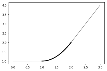
keep_slope

BpfInterface.keep_slope(self, double epsilon=0.0001)

A view of this bpf where the slope is continued outside its bounds

Return a new bpf which is a copy of this bpf when inside bounds() but outside bounds() it behaves as a linear bpf with a slope equal to the slope of this bpf at its extremes

Example

a = expon(1, 1, 2, 2, exp=2)
b = a.keep_slope()
b[0:3].plot(show=False, color="grey")
a.plot(color="black", linewidth=3)

Args

• epsilon (float): an epsilon value to use when deriving the this bpf to calculate its slope (default: 0.0001)

Returns

    (BpfInterface) A view of this bpf which keeps its slope outside its bounds (instead of just returning the last defined value)

---

log

BpfInterface.log(self, double base=M_E) -> _BpfLambdaLog

Returns a bpf representing the log of this bpf

Args

• base (float): the base of the log (default: 2.718281828459045)

Returns

    (BpfInterface) A bpf representing \x -> log(self(x), base)

---

log10

BpfInterface.log10(self) -> _BpfUnaryFunc

Returns a bpf representing the log10 of this bpf

---

m2f

BpfInterface.m2f(self, double a4=0.)

Returns a bpf converting from midinotes to frequency

Example

>>> from bpf4 import *
>>> midinotes = linear(0, 60, 1, 65)
>>> freqs = midinotes.m2f()
>>> freqs.map(10)
array([262.81477242, 271.38531671, 280.23535149, 289.37399111,
       298.81064715, 308.55503809, 318.61719934, 329.0074936 ,
       339.73662146, 350.81563248])

Args

• a4 (float): frequency value for A4. If not given, uses the global value (see setA4) (default: 0.0)

Returns

    (BpfInterface) A bpf representing \x -> m2f(self(x))

---

map

BpfInterface.map(self, xs, ndarray out=None) -> ndarray

The same as map(self, xs) but faster

bpf.map(10) == bpf.map(numpy.linspace(x0, x1, 10))

Example

>>> out = numpy.empty((100,), dtype=float)
>>> xs = numpy.linspace(0, 10, 100)
# This is the right way to pass an output array
>>> out = thisbpf.map(xs, out)   

Args

• xs (ndarray | int): the x coordinates at which to sample this bpf, or an integer representing the number of elements to calculate in an evenly spaced grid between the bounds of this bpf
• out (ndarray): if given, an attempt will be done to use it as destination for the result. The user should not trust that this actually happens (see example) (default: None)

---

mapn_between

BpfInterface.mapn_between(self, int n, double x0, double x1, ndarray out=None) -> ndarray

Calculate an array of n values representing this bpf between x0 and x1

x0 and x1 are included

Example

out = numpy.empty((100,), dtype=float)
out = thisbpf.mapn_between(100, 0, 10, out)

Args

• n:
• x0 (float): lower bound to map this bpf
• x1 (float): upper bound to map this bpf
• out (ndarray): if included, results are placed here. (default: None)

Returns

    (ndarray) An array of n elements representing this bpf at the given values within the range x0:x1. This is out if it was passed

---

max

BpfInterface.max(self, b)

Returns a bpf representing max(self, b)

Example

>>> from bpf4 import *
>>> a = linear(0, 0, 1, 10)
>>> b = a.max(4)
>>> b(0), b(0.5), b(1)
(4.0, 5.0, 10.0)
>>> b.plot()

Args

• b (float | BpfInterface): a const float or a bpf

Returns

    (Max) A Max bpf representing max(self, b), which can be evaluated at any x coord

---

mean

BpfInterface.mean(self) -> double

Calculate the mean value of this bpf.

To constrain the calculation to a given portion, use:

bpf.integrate_between(start, end) / (end-start)

Returns

    (float) The average value of this bpf along its bounds

---

min

BpfInterface.min(self, b)

Returns a bpf representing min(self, b)

Example

>>> from bpf4 import *
>>> a = linear(0, 0, 1, 10)
>>> b = a.min(4)
>>> b(0), b(0.5), b(1)
(0, 4.0, 5.0)
>>> b.plot()

Args

• b (float | BpfInterface): a const float or a bpf

Returns

    (Min) A Min bpf representing min(self, b), which can be evaluated at any x coord

---

nanmask

BpfInterface.nanmask(self, double masked=0.) -> NanMask

A nan mask from this bpf

A nan mask returns nan whenever this bpf returns the masked value, otherwise it returns its original value.

Example

Create a mask for a frequency bpf b, to set it to nan whenever the frequency is lower than 50 Hz

>>> b = bpf.linear(0, 440, 1, 440, 2, 100, 3, 40, 5, 80, 6, 440)
>>> bmasked = b * (b >= 50).nanmask()
>>> bmasked.plot()
>>> bpf4.util.split_fragments(bmasked)

Args

• masked (float): the value to convert to NAN (default: 0.0)

---

ntodx

BpfInterface.ntodx(self, int N) -> double

Calculate the sampling period dx

Calculate sampling period dx so that the bounds of this bpf are divided into N parts: dx = (x1-x0) / (N-1). The period is calculated so that lower and upper bounds are included, following numpy's linspace

!!! info "See Also"

 [dxton()](#dxton)

Example

---

```python

a = linear(0, 0, 1, 1) dx = a.ntodx(10) dx 0.11111111 np.arange(a.x0, a.x1, dx) array([0. , 0.11111111, 0.22222222, 0.33333333, 0.44444444, 0.55555556, 0.66666667, 0.77777778, 0.88888889, 1. ])

Args

• N (int): The number of points to sample within the bounds of this bpf

Returns

    (float) The sampling period dx

---

outbound

BpfInterface.outbound(self, double y0, y1=None)

Return a new Bpf with the given values outside the bounds

Used like bpf.outbound(0, 0) + fallbackbpf it can be used to give a fallback bpf for values outside this bpf (see example)

Examples

>>> from bpf4 import *
>>> a = linear(0, 1, 1, 10).outbound(-1, 0)
>>> a(-0.5)
-1
>>> a(1.1)
0
>>> a(0)
1
>>> a(1)
10

# fallback to another curve outside self
>>> a = linear(0, 1, 1, 10).outbound(0, 0) + expon(-1, 2, 4, 10, exp=2)
>>> a.plot()

Args

• y0 (float): returned for x values lower than the lower bound
• y1 (float): returned for x values higher than the upper bound. If not given, the same value for y0 is used (default: None)

Returns

    (BpfInterface) a bpf where inside the bounds it returns the values of this bpf and outside the bounds the values given here

---

periodic

BpfInterface.periodic(self)

Create a new bpf which replicates this in a periodic way

The new bpf is a copy of this bpf when inside its bounds and outside it, it replicates it in a periodic way, with no bounds.

Example

>>> from bpf4 import *
>>> a = core.Linear((0, 1), (-1, 1)).periodic()
>>> a
_BpfPeriodic[-inf:inf]
>>> a.plot()

Returns

    (BpfInterface) A periodic view of this bpf

---

plot

BpfInterface.plot(self, kind=u'line', int n=-1, show=True, axes=None, **keys)

Plot the bpf using matplotlib.pyplot. Any key is passed to plot.plot_coords

Example

from bpf4 import *
a = linear(0, 0, 1, 10, 2, 0.5)
a.plot()

# Plot to a preexistent axes
ax = plt.subplot()
a.plot(axes=ax)

Args

• kind (str): one of 'line', 'bar' (default: line)
• n (int): the number of points to plot (default: -1)
• show (bool): if the plot should be shown immediately after (default is True). If you want to display multiple BPFs sharing an axes you can call plot on each of the bpfs with show=False, and then either call the last one with plot=True or call bpf4.plot.show(). (default: True)
• axes (matplotlib.pyplot.Axes): if given, will be used to plot onto it, otherwise an ad-hoc axes is created (default: None)
• keys:

Returns

    the pyplot.Axes object. This will be the axes passed as argument, if given, or a new axes created for this plot

---

preapply

BpfInterface.preapply(self, func)

Create a bpf where func is applied to the argument before it is passed

This is equivalent to func(x) | self

Example

>>> bpf = Linear((0, 1, 2), (0, 10, 20))
>>> bpf(0.5)
5

>>> shifted_bpf = bpf.preapply(lambda x: x + 1)
>>> shifted_bpf(0.5)
15

NB: bpf1.preapply(bpf2) is the same as bpf2 | bpf1

Args

• func (callable): a function func(x: float) -> float which is applied to the argument before passing it to this bpf

Returns

    (BpfInterface) A bpf following the pattern lambda x: bpf(func(x))

---

rand

BpfInterface.rand(self) -> _BpfRand

A bpf representing rand(self(x))

Returns

    (BpfInterface) A bpf representing the operation `rand(self(x))

---

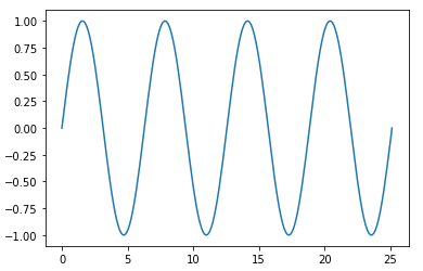
render

BpfInterface.render(self, xs, interpolation=u'linear')

Create a new bpf representing this bpf rendered at the given points

The difference between .render and .sampled is that this method creates a Linear/NoInterpol bpf whereas .sampled returns a Sampled bpf (a Sampled bpf works only for regularly sampled data, a Linear or NoInterpol bpfs accept any data as its x coordinate)

Example

>>> from bpf4 import *
>>> from math import *
>>> a = slope(1)[0:4*pi].sin()
>>> b = a.render(20)   # Sample this bpf at 20 points within its bounds
>>> b
Sampled[0.0:12.566370614359172]
>>> b.plot()

See Also

BpfInterface.sampled

Args

• xs (int | list | np.ndarray): a seq of points at which this bpf is sampled or a number, in which case an even grid is calculated with that number of points. In the first case a Linear or NoInterpol bpf is returned depending on the interpolation parameter (see below). In the second case a Sampled bpf is returned.
• interpolation (str): the interpoltation type of the returned bpf. One of 'linear', 'nointerpol' (default: linear)

Returns

    (BpfInterface) a new bpf representing this bpf. Depending on the interpolation this new bpf will be a Sampled, a Linear or a NoInterpol bpf

---

round

BpfInterface.round(self) -> _BpfLambdaRound

A bpf representing round(self(x))

Returns

    (BpfInterface) A bpf representing the operation round(self(x))

---

sample_between

BpfInterface.sample_between(self, double x0, double x1, double dx, ndarray out=None) -> ndarray

Sample this bpf at an interval of dx between x0 and x1

Note

The interface is similar to numpy's linspace

Example

>>> a = linear(0, 0, 10, 10)
>>> a.sample_between(0, 10, 1)
[0 1 2 3 4 5 6 7 8 9 10]

This is the same as a.mapn_between(11, 0, 10)

Args

• x0 (float): point to start sampling (included)
• x1 (float): point to stop sampling (included)
• dx (float): the sampling period
• out (ndarray): if given, the result will be placed here and no new array will be allocated (default: None)

Returns

    (ndarray) An array with the values of this bpf sampled at at a regular grid of period dx from x0 to x1. If out is given the result is placed in it

---

sampled

BpfInterface.sampled(self, double dx, interpolation=u'linear') -> BpfInterface

Sample this bpf at a regular interval, returns a Sampled bpf

Sample this bpf at an interval of dx (samplerate = 1 / dx) returns a Sampled bpf with the given interpolation between the samples

Note

If you need to sample a portion of the bpf, use sampled_between

The same results can be achieved via indexing, in which case the resulting bpf will be linearly interpolated:

bpf[::0.1]    # returns a sampled version of this bpf with a dx of 0.1
bpf[:10:0.1]  # samples this bpf between (x0, 10) at a dx of 0.1

See Also

ntodx, dxton

Args

• dx (float): the sample interval
• interpolation (str): the interpolation kind. One of 'linear', 'nointerpol', 'halfcos', 'expon(XX)', 'halfcos(XX)' (where XX is an exponential passed to the interpolation function) (default: linear)

Returns

    (Sampled) The sampled bpf

---

sampled_between

BpfInterface.sampled_between(self, double x0, double x1, double dx, interpolation=u'linear') -> BpfInterface

Sample a portion of this bpf, returns a Sampled bpf

NB: This is the same as thisbpf[x0:x1:dx]

Args

• x0 (float): point to start sampling (included)
• x1 (float): point to stop sampling (included)
• dx (float): the sampling period
• interpolation (str): the interpolation kind. One of 'linear', 'nointerpol', 'halfcos', 'expon(XX)', 'halfcos(XX)' (where XX is an exponential passed to the interpolation function). For (default: linear)

Returns

    (Sampled) The Sampled bpf, representing this bpf sampled at a grid of [x0:x1:dx] with the given interpolation

---

shifted

BpfInterface.shifted(self, dx) -> BpfInterface

Returns a view of this bpf shifted by dx over the x-axes

This is the same as .shift, but a new bpf is returned

Example

>>> from bpf4 import *
>>> a = linear(0, 1, 1, 5)
>>> b = a.shifted(2)
>>> b(3) == a(1)

Args

• dx:

---

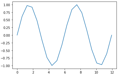
sin

BpfInterface.sin(self) -> _BpfUnaryFunc

Returns a bpf representing the sine of this bpf

from bpf4 import *
from math import pi
a = slope(1).sin()
a[0:8*pi].plot()

---

sinh

BpfInterface.sinh(self) -> _BpfUnaryFunc

Returns a bpf representing the sinh of this bpf

---

sqrt

BpfInterface.sqrt(self) -> _BpfUnaryFunc

Returns a bpf representing the sqrt of this bpf

---

stretched

BpfInterface.stretched(self, double rx, double fixpoint=0.)

Returns a view of this bpf stretched over the x axis.

NB: to stretch over the y-axis, just multiply this bpf

See Also

fit_between()

Example

Stretch the shape of the bpf, but preserve the start position

>>> a = linear(1, 1, 2, 2)
>>> b = a.stretched(4, fixpoint=a.x0)
>>> b.bounds()
(1, 9)
>>> a.plot(show=False); b.plot()

Args

• rx (float): the stretch factor
• fixpoint (float): the point to use as reference (default: 0.0)

Returns

    (BpfInterface) A projection of this bpf stretched/compressed by by the given factor

---

tan

BpfInterface.tan(self) -> _BpfUnaryFunc

Returns a bpf representing the tan of this bpf

---

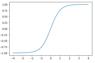
tanh

BpfInterface.tanh(self) -> _BpfUnaryFunc

Returns a bpf representing the tanh of this bpf

from bpf4 import *
a = slope(1).tanh()
a[-4:4].plot()

---

zeros

BpfInterface.zeros(self, double h=0.01, int N=0, double x0=NAN, double x1=NAN, int maxzeros=0) -> list

Find the zeros of this bpf

Example

>>> a = bpf.linear(0, -1, 1, 1)
>>> a.zeros()
[0.5]

Args

• h (float): the accuracy to scan for zero-crossings. If two zeros are within this distance, they will be resolved as one. (default: 0.01)
• N (int): alternatively, you can give the number of intervals to scan. h will be derived from this (default: 0)
• x0 (float): the point to start searching. If not given, the starting point of this bpf will be used (default: nan)
• x1 (float): the point to stop searching. If not given, the end point of this bpf is used (default: nan)
• maxzeros (int): if > 0, stop the search when this number of zeros have been found (default: 0)

Returns

    (List[float]) A list with the zeros of this bpf

---

BpfBase

• Base Class: BpfInterface

BpfBase(xs, ys)

---

Summary

Property	Description
descriptor	BpfBase.descriptor: str

    A string describing the interpolation function of this bpf |

| exp | BpfBase.exp: float

    The exponential of the interpolation function of this bpf |

Method	Description
init	Base constructor for bpfs
clone_with_new_data	Create a new bpf with the same attributes as self but with new data
insertpoint	Return a copy of this bpf with the point (x, y) inserted
mapn_between	BpfBase.mapn_between(self, int n, double xstart, double xend, ndarray out=None) -> ndarray
outbound	Set the values inplace returned when this bpf is evaluated outside its bounds.
points	Returns a tuple with the points defining this bpf
removepoint	Return a copy of this bpf with point at x removed
segments	Return an iterator over the segments of this bpf
shift	Shift the bpf along the x-coords, INPLACE
split	Split this bpf into fragments separated by nan y values
stretch	Stretch or compress this bpf in the x-coordinate INPLACE

---

Attributes

• descriptor: BpfBase.descriptor: str A string describing the interpolation function of this bpf
• exp: BpfBase.exp: float The exponential of the interpolation function of this bpf

---

Methods

__init__

def __init__(xs: list[float] | numpy.ndarray, ys: list[float] | numpy.ndarray
             ) -> None

Base constructor for bpfs

xs and ys should be of the same size

Args

• xs (list[float] | numpy.ndarray): x data
• ys (list[float] | numpy.ndarray): y data

---

clone_with_new_data

BpfBase.clone_with_new_data(self, ndarray xs: ndarray, ndarray ys: ndarray) -> BpfInterface

Create a new bpf with the same attributes as self but with new data

Args

• xs (ndarray): the x-coord data
• ys (ndarray): the y-coord data

Returns

    (BpfInterface) The new bpf. It will be of the same class as self

---

insertpoint

BpfBase.insertpoint(self, double x, double y)

Return a copy of this bpf with the point (x, y) inserted

Note

self is not modified

Args

• x (float): x coord
• y (float): y coord

Returns

    (BpfInterface) A clone of this bpf with the point inserted

---

mapn_between

def mapn_between(self, n, xstart, xend, out=None) -> None

BpfBase.mapn_between(self, int n, double xstart, double xend, ndarray out=None) -> ndarray

Args

• n:
• xstart:
• xend:
• out: (default: None)

---

outbound

BpfBase.outbound(self, double y0, y1=None)

Set the values inplace returned when this bpf is evaluated outside its bounds.

The default behaviour is to interpret the values at the bounds to extend to infinity. In order to not change this bpf inplace, use b.copy().outbound(y0, y1)

Args

• y0 (float): the value for the lower bound
• y1 (float | None): the value for the upper bound (y0 if not given) (default: None)

Returns

    (BpfInterface) self

---

points

BpfBase.points(self)

Returns a tuple with the points defining this bpf

Example

>>> b = Linear.fromseq(0, 0, 1, 100, 2, 50)
>>> b.points()
([0, 1, 2], [0, 100, 50])

Returns

    (tuple[ndarray, ndarray]) a tuple (xs, ys) where xs is an array holding the values for the x coordinate, and ys holds the values for the y coordinate

---

removepoint

BpfBase.removepoint(self, double x)

Return a copy of this bpf with point at x removed

Raises ValueError if x is not in this bpf

To remove elements by index, do:

xs, ys = mybpf.points()
xs = numpy.delete(xs, indices)
ys = numpy.delete(ys, indices)
mybpf = mybpf.clone_with_new_data(xs, ys)

Args

• x (float): the x point to remove

Returns

    (BpfInterface) A copy of this bpf with the given point removed

---

segments

BpfBase.segments(self)

Return an iterator over the segments of this bpf

Each segment is a tuple (x: float, y: float, interpoltype: str, exponent: float)

Exponent is only of value if the interpolation type makes use of it.

Returns

    (Iterable[tuple[float, float, str, float]]) An iterator of segments, where each segment has the form (x, y, interpoltype:str, exponent)

---

shift

BpfBase.shift(self, double dx)

Shift the bpf along the x-coords, INPLACE

Use .shifted to create a new bpf

Args

• dx (float): the shift interval

---

split

BpfBase.split(self, double sep=NAN)

Split this bpf into fragments separated by nan y values

Args

• sep (float): the separator to use (default: nan)

Returns

    (list[BpfBase]) A list of fragments

---

stretch

BpfBase.stretch(self, double rx)

Stretch or compress this bpf in the x-coordinate INPLACE

NB: use stretched to create a new bpf

Args

• rx (float): the stretch/compression factor

---

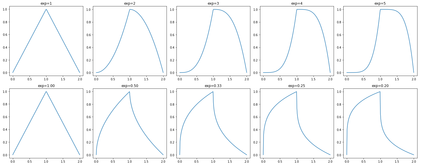
Expon

• Base Class: BpfBase

Expon(xs, ys, double exp, int numiter=1)

A bpf with exponential interpolation

Example

from bpf4 import *
import matplotlib.pyplot as plt
numplots = 5
fig, axs = plt.subplots(2, numplots, tight_layout=True, figsize=(20, 8))
for i in range(numplots):
    exp = i+1
    core.Expon([0, 1, 2], [0, 1, 0], exp=exp).plot(show=False, axes=axs[0, i])
    core.Expon([0, 1, 2], [0, 1, 0], exp=1/exp).plot(show=False, axes=axs[1, i])
    axs[0, i].set_title(f'{exp=}')
    axs[1, i].set_title(f'exp={1/exp:.2f}')

plot.show()

---

Summary

Method	Description
init	-

---

---

Methods

__init__

def __init__(xs: ndarray, ys: ndarray, exp: float, numiter: int) -> None

Args

• xs (ndarray): the x-coord data
• ys (ndarray): the y-coord data
• exp (float): an exponent applied to the halfcosine interpolation
• numiter (int): how many times to apply the interpolation

---

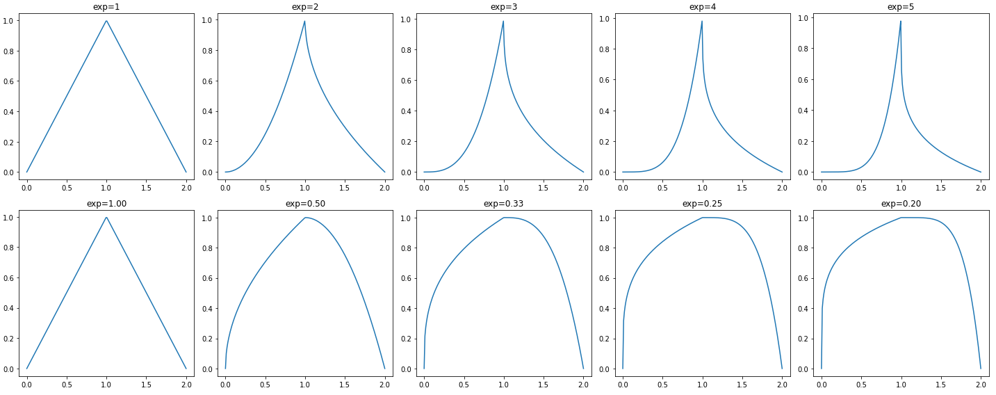
Exponm

• Base Class: Expon

Exponm(xs, ys, double exp, int numiter=1)

A bpf with symmetrical exponential interpolation

from bpf4 import *
import matplotlib.pyplot as plt
numplots = 5
fig, axs = plt.subplots(2, numplots, tight_layout=True, figsize=(20, 8))
for i in range(numplots):
    exp = i+1
    core.Exponm([0, 1, 2], [0, 1, 0], exp=exp).plot(show=False, axes=axs[0, i])
    core.Exponm([0, 1, 2], [0, 1, 0], exp=1/exp).plot(show=False, axes=axs[1, i])
    axs[0, i].set_title(f'{exp=}')
    axs[1, i].set_title(f'exp={1/exp:.2f}')

plot.show()

---

Summary

Method	Description
init	-

---

---

Methods

__init__

def __init__(xs: ndarray, ys: ndarray, exp: float, numiter: int) -> None

Args

• xs (ndarray): the x-coord data
• ys (ndarray): the y-coord data
• exp (float): an exponent applied to the halfcosine interpolation
• numiter (int): how many times to apply the interpolation

---

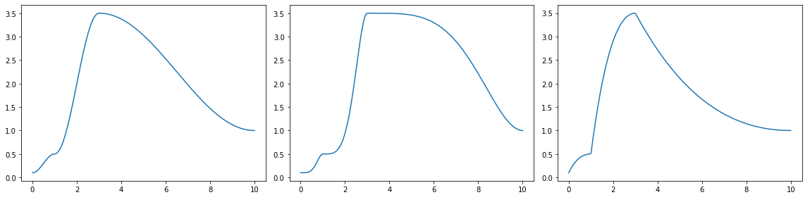
Halfcos

• Base Class: BpfBase

Halfcos(xs, ys, double exp=1.0, int numiter=1)

A bpf with half-cosine interpolation

HalfcosExp is the same as Halfcos. It exists with two names for compatibility

a = core.Halfcos([0, 1, 3, 10], [0.1, 0.5, 3.5,  1])
b = core.Halfcos(*a.points(), exp=2)
c = core.Halfcos(*a.points(), exp=0.5)
fig, axes = plt.subplots(1, 3, figsize=(16, 4), tight_layout=True)
a.plot(axes=axes[0], show=False)
b.plot(axes=axes[1], show=False)
c.plot(axes=axes[2])

---

Summary

Method	Description
init	-

---

---

Methods

__init__

def __init__(xs: ndarray, ys: ndarray, exp: float, numiter: int) -> None

Args

• xs (ndarray): the x-coord data
• ys (ndarray): the y-coord data
• exp (float): an exponent applied to the halfcosine interpolation
• numiter (int): how many times to apply the interpolation

---

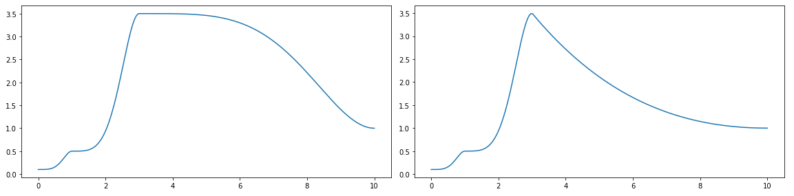
Halfcosm

• Base Class: Halfcos

Halfcosm(xs, ys, double exp=1.0, int numiter=1)

A bpf with half-cosine and exponent depending on the orientation of the interpolation

When interpolating between two y values, y0 and y1, if y1 < y0 the exponent is inverted, resulting in a symmetrical interpolation shape

a = core.Halfcos([0, 1, 3, 10], [0.1, 0.5, 3.5,  1], exp=2)
b = core.Halfcosm(*a.points(), exp=2)
fig, axes = plt.subplots(1, 2, figsize=(16, 4))
a.plot(axes=axes[0], show=False)
b.plot(axes=axes[1])

---

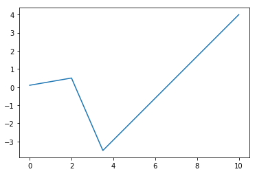
Linear

• Base Class: BpfBase

Linear(xs, ys)

A bpf with linear interpolation

from bpf4 import *
a = core.Linear([0, 2, 3.5, 10], [0.1, 0.5, -3.5,  4])
a.plot()

---

Summary

Method	Description
init	-
flatpairs	Returns a flat 1D array with x and y values interlaced
integrate_between	Integrate this bpf between the given x coords
inverted	Return a new Linear bpf where x and y coordinates are inverted.
simplify	Simplify this bpf
sliced	Cut this bpf at the given points

---

---

Methods

__init__

def __init__(xs: ndarray, ys: ndarray) -> None

Args

• xs (ndarray): the x-coord data
• ys (ndarray): the y-coord data

---

flatpairs

Linear.flatpairs(self)

Returns a flat 1D array with x and y values interlaced

>>> a = linear(0, 0, 1, 10, 2, 20)
>>> a.flatpairs()
array([0, 0, 1, 10, 2, 20])

Returns

    (ndarray) A 1D array representing the points of this bpf with xs and ys interleaved

---

integrate_between

Linear.integrate_between(self, double x0, double x1, size_t N=0) -> double

Integrate this bpf between the given x coords

Args

• x0 (float): start of integration
• x1 (float): end of integration
• N (int): number of integration steps (default: 0)

Returns

    (float) The result representing the area beneath the curve between x0 and x1

---

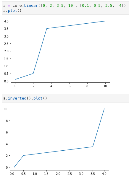
inverted

Linear.inverted(self)

Return a new Linear bpf where x and y coordinates are inverted.

This is only possible if y never decreases in value. Otherwise a ValueError is thrown

Returns

    (Linear) The inverted bpf

---

simplify

Linear.simplify(self, threshold=0., ratio=0.) -> Linear

Simplify this bpf

Either threshold or ratio must be given, but not both

Args

• threshold (float): the simplification threshold (default: 0.0)
• ratio (float): the simplification ratio. If given, simplification is done by ratio, the higher this value the more the shape is simplified (default: 0.0)

Returns

    (Linear) a new Linear bpf with its points simplified by the given parameter. Notice that the start and end points are never simplified

---

sliced

Linear.sliced(self, double x0, double x1) -> Linear

Cut this bpf at the given points

If needed it inserts points at the given coordinates to limit this bpf to the range x0:x1.

NB: this is different from crop, which is just a "view" into the underlying bpf. In this case a real Linear bpf is returned.

Args

• x0 (float): start x to cut
• x1 (float): end x to cut

Returns

    (Linear) Copy of this bpf cut at the given x-coords

---

Nearest

• Base Class: BpfBase

Nearest(xs, ys)

A bpf with nearest interpolation

a = core.Linear([0, 1, 3, 10], [0.1, 0.5, 3.5,  1])
b = core.NoInterpol(*a.points())
c = core.Nearest(*a.points())
fig, axes = plt.subplots(1, 3, figsize=(15, 4), tight_layout=True)
a.plot(axes=axes[0], show=False)
b.plot(axes=axes[1], show=False)
c.plot(axes=axes[2])

---

Summary

Method	Description
init	A bpf with nearest interpolation

---

---

Methods

__init__

def __init__(xs: ndarray, ys: ndarray) -> None

A bpf with nearest interpolation

Args

• xs (ndarray): the x coord data
• ys (ndarray): the y coord data

---

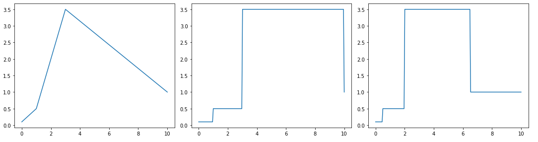
NoInterpol

• Base Class: BpfBase

NoInterpol(xs, ys)

A bpf without interpolation

a = core.Linear([0, 1, 3, 10], [0.1, 0.5, 3.5,  1])
b = core.NoInterpol(*a.points())
c = core.Nearest(*a.points())
fig, axes = plt.subplots(1, 3, figsize=(15, 4), tight_layout=True)
a.plot(axes=axes[0], show=False)
b.plot(axes=axes[1], show=False)
c.plot(axes=axes[2])

---

Summary

Method	Description
init	A bpf without interpolation

---

---

Methods

__init__

def __init__(xs: ndarray, ys: ndarray) -> None

A bpf without interpolation

Args

• xs (ndarray): the x coord data
• ys (ndarray): the y coord data

---

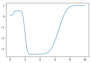
Smooth

• Base Class: BpfBase

Smooth(xs, ys, int numiter=1)

A bpf with smoothstep interpolation.

>>> a = Smooth([0, 1, 3, 10], [0.1, 0.5, -3.5,  1])
>>> a.plot()

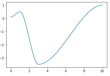
>>> a = core.Smooth([0, 1, 3, 10], [0.1, 0.5, -3.5,  1], numiter=3)
>>> a.plot()

---

Summary

Method	Description
init	-

---

---

Methods

__init__

def __init__(xs: ndarray, ys: ndarray, numiter: int) -> None

Args

• xs (ndarray): the x-coord data
• ys (ndarray): the y-coord data
• numiter (int): the number of smoothstep steps

---

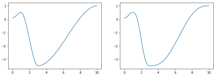
Smoother

• Base Class: BpfBase

Smoother(xs, ys)

A bpf with smootherstep interpolation (perlin's variation of smoothstep)

a = core.Smooth([0, 1, 3, 10], [0.1, 0.5, -3.5,  1])
b = core.Smoother(*a.points())
fig, axes = plt.subplots(1, 2, figsize=(12, 4))
a.plot(axes=axes[0], show=False)
b.plot(axes=axes[1])

---

Const

• Base Class: BpfInterface

Const(double value, tuple bounds: tuple[float, float] = None)

A bpf representing a constant value

---

Summary

Method	Description
init	-
mapn_between	Const.mapn_between(self, int n, double x0, double x1, ndarray out=None) -> ndarray

---

---

Methods

__init__

def __init__(value: float) -> None

Args

• value (float): the constant value of this bpf

---

mapn_between

def mapn_between(self, n, x0, x1, out=None) -> None

Const.mapn_between(self, int n, double x0, double x1, ndarray out=None) -> ndarray

Args

• n:
• x0:
• x1:
• out: (default: None)

---

Multi

• Base Class: BpfInterface

Multi(xs, ys, interpolations)

A bpf where each segment can have its own interpolation kind

---

Summary

Method	Description
init	!!! note
segments	Returns an iterator over the segments of this bpf

---

---

Methods

__init__

def __init__(xs: ndarray, ys: ndarray, interpolations: list[str]) -> None

Note

Note

len(interpolations) == len(xs) - 1

The interpelation is indicated via a descriptor: 'linear' (linear), 'expon(x)' (exponential with exp=x), 'halfcos', 'halfcos(x)' (cosine interpol with exp=x), 'nointerpol', `'smooth' (smoothstep)

Args

• xs (ndarray): the sequence of x points
• ys (ndarray): the sequence of y points
• interpolations (list[str]): the interpolation used between these points

---

segments

Multi.segments(self)

Returns an iterator over the segments of this bpf

Returns

    (Iterator[tuple[float, float, str, float]]) An iterator of segments, where each segment has the form (x, y, interpoltype:str, exponent)

---

Sampled

• Base Class: BpfInterface

Sampled(samples, double dx, double x0=0, unicode interpolation=u'linear')

A bpf with regularly sampled data

When evaluated, values between the samples are interpolated with a given function: linear, expon(x), halfcos, halfcos(x), etc.

---

Summary

Property	Description
dx	Sampled.dx: float

    The sampling period (delta x) |

| interpolation | - | | samplerate | Sampled.samplerate: float

    The samplerate of this bpf |

| xs | Sampled.xs: numpy.ndarray

    The x-coord array of this bpf |

| ys | - |

Method	Description
init	-
aslinear	A linear version of this bpf
derivative	Return a curve which represents the derivative of this curve
flatpairs	Returns a flat 1D array with x and y values interlaced
integrate	Return the result of the integration of this bpf.
integrate_between	The same as integrate() but between the (included) bounds x0-x1
inverted	Return a view on this bpf with the coords inverted
mapn_between	Return an array of n elements resulting of evaluating this bpf regularly
points	Returns a tuple with the points defining this bpf
segments	Returns an iterator over the segments of this bpf
set_interpolation	Sets the interpolation of this Sampled bpf, inplace
split	Split this Sampled bpf into fragments separated by nan y values

---

Attributes

• dx: Sampled.dx: float The sampling period (delta x)
• interpolation
• samplerate: Sampled.samplerate: float The samplerate of this bpf
• xs: Sampled.xs: numpy.ndarray The x-coord array of this bpf
• ys

---

Methods

__init__

def __init__(samples: ndarray, dx: float, x0: float, interpolation: str) -> None

Args

• samples (ndarray): the y-coord sampled data
• dx (float): the sampling period
• x0 (float): the first x-value
• interpolation (str): the interpolation function used. One of 'linear', 'nointerpol', 'expon(X)', 'halfcos', 'halfcos(X)', 'smooth', 'halfcosm', etc.

---

aslinear

Sampled.aslinear(self, simplify=0.)

A linear version of this bpf

Args

• simplify (float): (default: 0.0)

---

derivative

Sampled.derivative(self) -> BpfInterface

Return a curve which represents the derivative of this curve

It implements Newtons difference quotiont, so that:

derivative(x) = bpf(x + h) - bpf(x)
                -------------------
                          h

Example

>>> from bpf4 import *
>>> a = slope(1)[0:6.28].sin()
>>> a.plot(show=False, color="red")
>>> b = a.derivative()
>>> b.plot(color="blue")

---

flatpairs

Sampled.flatpairs(self)

Returns a flat 1D array with x and y values interlaced

>>> a = linear(0, 0, 1, 10, 2, 20)
>>> a.flatpairs()
array([0, 0, 1, 10, 2, 20])

Returns

    (ndarray) A 1D array with x and y values interlaced

---

integrate

Sampled.integrate(self) -> double

Return the result of the integration of this bpf.

If any of the bounds is inf, the result is also inf.

NB: to determine the limits of the integration, first crop the bpf via a slice

Example

Integrate this bpf from its lower bound to 10 (inclusive)

b[:10].integrate()  

---

integrate_between

Sampled.integrate_between(self, double x0, double x1, size_t N=0) -> double

The same as integrate() but between the (included) bounds x0-x1

It is effectively the same as bpf[x0:x1].integrate(), but more efficient

NB: N has no effect. It is put here to comply with the signature of the function.

Args

• x0:
• x1:
• N (int): (default: 0)

---

inverted

Sampled.inverted(self)

Return a view on this bpf with the coords inverted

In an inverted function the coordinates are swaped: the inverted version of a bpf indicates which x corresponds to a given y

Returns None if the function is not invertible. For a function to be invertible, it must be strictly increasing or decreasing, with no local maxima or minima.

f.inverted()(f(x)) = x

So if y(1) == 2, then y.inverted()(2) == 1

Returns

    (BpfInterface) a view on this bpf with the coords inverted

---

mapn_between

Sampled.mapn_between(self, int n, double x0, double x1, ndarray out=None) -> ndarray

Return an array of n elements resulting of evaluating this bpf regularly

The x coordinates at which this bpf is evaluated are equivalent to linspace(xstart, xend, n)

Args

• n (int): the number of elements to generate
• x0 (float): x to start mapping
• x1 (float): x to end mapping
• out (ndarray): if given, result is put here (default: None)

Returns

    (ndarray) An array of this bpf evaluated at a grid [xstart:xend:dx], where dx is (xend-xstart)/n

---

points

Sampled.points(self)

Returns a tuple with the points defining this bpf

Example

>>> b = Linear.fromseq(0, 0, 1, 100, 2, 50)
>>> b.points()
([0, 1, 2], [0, 100, 50])

Returns

    (tuple[ndarray, ndarray]) A tuple (xs, ys) where xs is an array holding the values for the x coordinate, and ys holds the values for the y coordinate

---

segments

Sampled.segments(self)

Returns an iterator over the segments of this bpf

Each item is a tuple (float x, float y, str interpolation_type, float exponent)

NB: exponent is only relevant if the interpolation type makes use of it

Returns

    (Iterable[tuple[float, float, str, float]]) An iterator of segments, where each segment has the form (x, y, interpoltype:str, exponent)

---

set_interpolation

Sampled.set_interpolation(self, unicode interpolation) -> Sampled

Sets the interpolation of this Sampled bpf, inplace

Returns self, so you can do:

sampled = bpf[x0:x1:dx].set_interpolation('expon(2)')

Args

• interpolation (str): the interpolation kind

Returns

    (Sampled) self

---

split

Sampled.split(self, double sep=NAN)

Split this Sampled bpf into fragments separated by nan y values

Args

• sep (float): the separator to use (default: nan)

Returns

    (list[Sampled]) A list of fragments

---

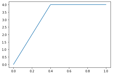
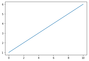
Slope

• Base Class: BpfInterface

Slope(double slope, double offset=0, tuple bounds=None)

A bpf representing a linear equation y = slope * x + offset

>>> from bpf4.core import *
>>> a = Slope(0.5, 1)
>>> a
Slope[-inf:inf]
>>> a[0:10].plot()

---

Summary

Property	Description
offset	offset: 'double'
slope	slope: 'double'

Method	Description
init	A bpf representing a linear equation y = slope * x + offset
mapn_between	Return an array of n elements resulting of evaluating this bpf regularly

---

Attributes

• offset: offset: 'double'
• slope: slope: 'double'

---

Methods

__init__

def __init__(slope: float, offset: float, bounds: tuple) -> None

A bpf representing a linear equation y = slope * x + offset

Args

• slope (float): the slope of the line
• offset (float): an offset added
• bounds (tuple): if given, the line is clipped on the x axis to the given bounds

---

mapn_between

Slope.mapn_between(self, int n, double x0, double x1, ndarray out=None) -> ndarray

Return an array of n elements resulting of evaluating this bpf regularly

The x coordinates at which this bpf is evaluated are equivalent to linspace(x0, 1, n)

Args

• n (int): the number of elements to generate
• x0 (float): x to start mapping
• x1 (float): x to end mapping
• out (ndarray): if given, result is put here (default: None)

Returns

    (ndarray) An array of this bpf evaluated at a grid [x0:x1:dx], where dx is (xend-xstart)/n

---

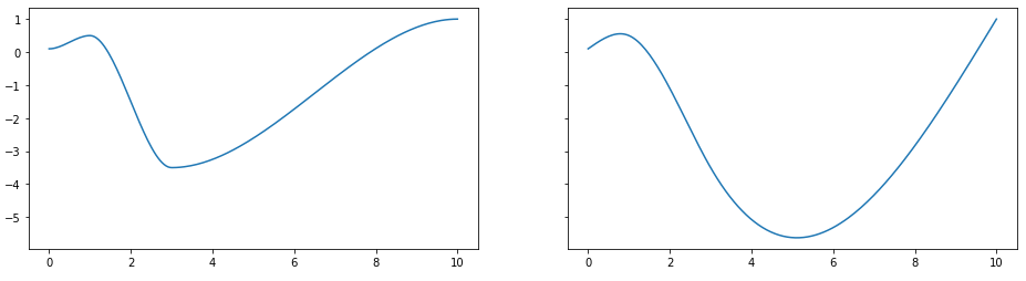
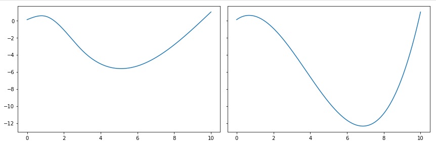
Spline

• Base Class: BpfInterface

Spline(xs, ys)

A bpf with cubic spline interpolation

With cubic spline interpolation, for each point (x, y) it is ensured that bpf(x) == y. Between the defined points, depending on their proximity, this bpf can overshoot

Example

a = core.Smooth([0, 1, 3, 10], [0.1, 0.5, -3.5,  1])
b = core.Spline(*a.points())
fig, axes = plt.subplots(1, 2, figsize=(12, 4))
a.plot(axes=axes[0], show=False)
b.plot(axes=axes[1])

---

Summary

Method	Description
init	A bpf with cubic spline interpolation
points	Returns a tuple with the points defining this bpf
segments	Returns an iterator over the segments of this bpf

---

---

Methods

__init__

def __init__(xs: ndarray, ys: ndarray) -> None

A bpf with cubic spline interpolation

Args

• xs (ndarray): the x coord data
• ys (ndarray): the y coord data

---

points

Spline.points(self)

Returns a tuple with the points defining this bpf

Example

>>> b = Linear.fromseq(0, 0, 1, 100, 2, 50)
>>> b.points()
([0, 1, 2], [0, 100, 50])

Returns

    (tuple[ndarray, ndarray]) a tuple (xs, ys) where xs is an array holding the values for the x coordinate, and ys holds the values for the y coordinate

---

segments

Spline.segments(self)

Returns an iterator over the segments of this bpf

Each segment is a tuple (float x, float y, str interpolation_type, float exponent)

Note

Exponent is only relevant if the interpolation type makes use of it

Returns

    (Iterable[tuple[float, float, str, float]]) An iterator of segments, where each segment has the form (x, y, interpoltype:str, exponent)

---

USpline

• Base Class: BpfInterface

USpline(xs, ys)

bpf with univariate spline interpolation.

a = core.Spline([0, 1, 3, 10], [0.1, 0.5, -3.5,  1])
b = core.USpline(*a.points())

fig, axes = plt.subplots(1, 2, figsize=(12, 4), sharey=True, tight_layout=True)
a.plot(axes=axes[0], show=False)
b.plot(axes=axes[1])

---

Summary

Method	Description
init	-
map	USpline.map(self, xs, ndarray out=None) -> ndarray
mapn_between	Return an array of n elements resulting of evaluating this bpf regularly
segments	Returns an iterator over the segments of this bpf

---

---

Methods

__init__

def __init__(xs: ndarray, ys: ndarray) -> None

Args

• xs (ndarray): the x coord data
• ys (ndarray): the y coord data

---

map

def map(self, xs, out=None) -> None

USpline.map(self, xs, ndarray out=None) -> ndarray

Args

• xs:
• out: (default: None)

---

mapn_between

USpline.mapn_between(self, int n, double x0, double x1, ndarray out=None) -> ndarray

Return an array of n elements resulting of evaluating this bpf regularly

The x coordinates at which this bpf is evaluated are equivalent to linspace(x0, x1, n)

Args

• n (int): the number of elements to generate
• x0 (float): x to start mapping
• x1 (float): x to end mapping
• out (ndarray): if given, result is put here (default: None)

Returns

    (ndarray) An array of this bpf evaluated at a grid [xstart:xend:dx], where dx is (xend-xstart)/n

---

segments

USpline.segments(self)

Returns an iterator over the segments of this bpf

Returns

    (Iterable[tuple[float, float, str, float]]) An iterator of segments, where each segment has the form (x, y, interpoltype:str, exponent)

---

_BpfUnaryOp

• Base Class: BpfInterface

_BpfUnaryOp(BpfInterface a)

A bpf representing a unary operation on a bpf

---

Summary

Method	Description
map	the same as map(self, xs) but somewhat faster
mapn_between	_BpfUnaryOp.mapn_between(self, int n, double x0, double x1, ndarray out=None) -> ndarray

---

---

Methods

map

_BpfUnaryOp.map(self, xs, ndarray out=None) -> ndarray

the same as map(self, xs) but somewhat faster

xs can also be a number, in which case it is interpreted as the number of elements to calculate in an evenly spaced grid between the bounds of this bpf. bpf.map(10) == bpf.map(numpy.linspace(x0, x1, 10)) ( this is the same as bpf.mapn_between(10, bpf.x0, bpf.x1) )

Args

• xs:
• out: (default: None)

---

mapn_between

def mapn_between(self, n, x0, x1, out=None) -> None

_BpfUnaryOp.mapn_between(self, int n, double x0, double x1, ndarray out=None) -> ndarray

Args

• n:
• x0:
• x1:
• out: (default: None)

---

NanMask

• Base Class: _BpfUnaryOp

NanMask(BpfInterface a, double masked=0.)

---

_MultipleBpfReduce

• Base Class: _MultipleBpfs

---

Summary

Method	Description
mapn_between	_MultipleBpfReduce.mapn_between(self, int n, double x0, double x1, ndarray out=None) -> ndarray

---

---

Methods

mapn_between

def mapn_between(self, n, x0, x1, out=None) -> None

_MultipleBpfReduce.mapn_between(self, int n, double x0, double x1, ndarray out=None) -> ndarray

Args

• n:
• x0:
• x1:
• out: (default: None)

---

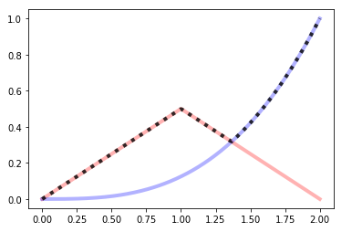
Max

• Base Class: _MultipleBpfReduce

Max(*bpfs)

A bpf which returns the max of multiple bpfs at a given point

a = linear(0, 0, 1, 0.5, 2, 0)
b = expon(0, 0, 2, 1, exp=3)
a.plot(show=False, color="red", linewidth=4, alpha=0.3)
b.plot(show=False, color="blue", linewidth=4, alpha=0.3)
core.Max((a, b)).plot(color="black", linewidth=4, alpha=0.8, linestyle='dotted')

---

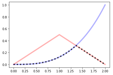
Min

• Base Class: _MultipleBpfReduce

Min(*bpfs)

A bpf which returns the min of multiple bpfs at a given point

a = linear(0, 0, 1, 0.5, 2, 0)
b = expon(0, 0, 2, 1, exp=3)
a.plot(show=False, color="red", linewidth=4, alpha=0.3)
b.plot(show=False, color="blue", linewidth=4, alpha=0.3)
core.Min((a, b)).plot(color="black", linewidth=4, alpha=0.8, linestyle='dotted')

---

_MultipleBpfs

• Base Class: BpfInterface

_MultipleBpfs(bpfs)

---

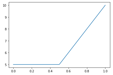
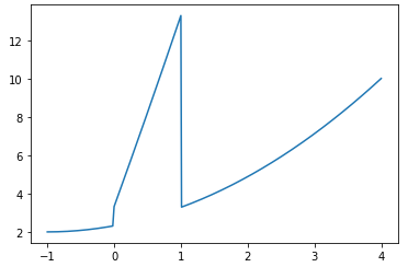
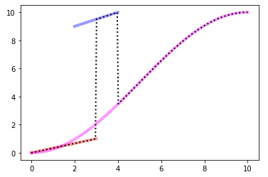
Stack

• Base Class: _MultipleBpfs

Stack(bpfs)

A bpf representing a stack of bpf

Within a Stack, a bpf does not have outbound values. When evaluated outside its bounds the bpf below is used, iteratively until the lowest bpf is reached. Only the lowest bpf is evaluated outside its bounds

Example

# Interval    bpf
# [0, 3]      a
# (3, 4]      b
# (4, 10]     c

from bpf4 import *
import matplotlib.pyplot as plt

a = linear(0, 0, 3, 1)
b = linear(2, 9, 4, 10)
c = halfcos(0, 0, 10, 10)
s = core.Stack((a, b, c))

ax = plt.subplot(111)
a.plot(color="#f00", alpha=0.4, axes=ax, linewidth=4, show=False)
b.plot(color="#00f", alpha=0.4, axes=ax, linewidth=4, show=False)
c.plot(color="#f0f", alpha=0.4, axes=ax, linewidth=4, show=False)
s.plot(axes=ax, linewidth=2, color="#000", linestyle='dotted')

---

Summary

Method	Description
init	-

---

---

Methods

__init__

def __init__(bpfs: list|tuple) -> None

Args

• bpfs (list|tuple): A sequence of bpfs. The order defined the evaluation order. The first bpf is on top, the last bpf is on bottom. Only the last bpf is evaluated outside its bounds

---

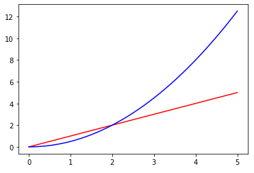
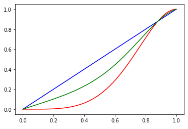
blend

blend(a, b, mix=0.5) -> BpfInterface

Blend these BPFs

Note

if mix == 0: the result is a if mix == 1: the result is b

Example

Create a curve which is in between a halfcos and a linear interpolation

from bpf4 import *
a = halfcos(0, 0, 1, 1, exp=2)
b = linear(0, 0, 1, 1)
c = blend(a, b, 0.5)

a.plot(show=False, color="red")
b.plot(show=False, color="blue")
c.plot(color="green")

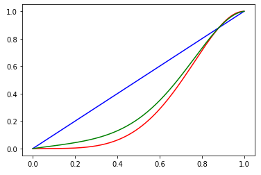
Closer to halfcos

c = blend(a, b, 0.2)
a.plot(show=False, color="red")
b.plot(show=False, color="blue")
c.plot(color="green")

Args

• a (BpfInterface): first bpf
• b (BpfInterface): second bpf
• mix (float): how to mix the bpfs. Can be fixed or itself a bpf (or any function) returning a value between 0-1 (default: 0.5)

Returns

    (BpfInterface) The blended bpf

---

bpf_zero_crossings

bpf_zero_crossings(BpfInterface b, double h=0.01, int N=0, double x0=NAN, double x1=NAN, int maxzeros=0) -> list

Return the zeros if b in the interval defined

Args

• b (BpfInterface): a bpf
• h (float): the interval to scan for zeros. for each interval only one zero will be found (default: 0.01)
• N (int): alternatively you can give the number of intervals to scan. h will be calculated from N (the h parameter is not used) (default: 0)
• x0 (float): If given, the bounds to search within (default: nan)
• x1 (float): If given, the bounds to search within (default: nan)
• maxzeros (int): if given, search will stop if this number of zeros is found (default: 0)

Returns

    (List[float]) A list of zeros (x coord points where the bpf is 0)

---

brentq

brentq(bpf, double x0, double xa, double xb, double xtol=9.9999999999999998e-13, double rtol=4.4408920985006262e-16, max_iter=100)

Calculate the zero of bpf + x0 in the interval (xa, xb) using brentq algorithm

Note

To calculate all the zeros of a bpf, use .zeros()

Example

# calculate the x where a == 0.5
>>> from bpf4 import *
>>> a = linear(0, 0, 10, 1)
>>> xzero, numcalls = brentq(a, -0.5, 0, 1)
>>> xzero
5

Args

• bpf (BpfInterface): the bpf to evaluate
• x0 (float): an offset so that bpf(x) + x0 = 0
• xa (float): the starting point to look for a zero
• xb (float): the end point
• xtol (float): The computed root x0 will satisfy np.allclose(x, x0, atol=xtol, rtol=rtol) (default: 1e-12)
• rtol (float): The computed root x0 will satisfy np.allclose(x, x0, atol=xtol, rtol=rtol) (default: 4.440892098500626e-16)
• max_iter (int): the max. number of iterations (default: 100)

Returns

    (tuple[float, int]) A tuple (zero of the bpf, number of function calls)

---

setA4

setA4(double freq)

Set the reference freq used

Args

• freq (float): the reference frequency for A4